Khanrc
AutoML (4) - DARTS: tutorial
Tutorial
Disclaimer
- 아래 코드 블럭들은 컨셉상 중요한 부분만 가져왔으니, 전체 코드가 궁금할 시 코드 블럭 상단의 링크를 참조.
- DARTS 는 퍼포먼스 (속도) 가 중요한 논문이라서 최대한 readability 를 고려하여 구현하였으나 퍼포먼스 이슈로 조금 복잡한 부분들이 존재한다.
- 원 저자의 코드를 많이 참조하였다.
본 글은 0.1 version 을 기준으로 작성되었음. 현재 마스터 브랜치의 최신 코드와는 일부 다를 수 있음.
Overview
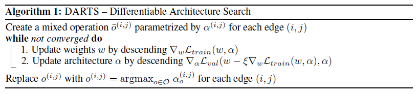
위 알고리즘 수도코드를 line by line 으로 옮기면:
- mixed operation 과 그 가중치 alpha 를 생성
- w 를 1-step 학습
- alpha 를 1-step 학습
- 수렴하면 alpha 의 큰 값들만 골라서 discrete 한 구조의 네트워크로 변환
1. Mixed op 및 alpha 생성
Mixed op 는 모든 후보 연산들이 믹스되어 있는 연산이다. 이 mixed op 가 모여서 DAG 로 표현되는 하나의 cell 이 되고, 이 cell 이 모여서 네트워크를 이룬다. 각 셀들은 셀의 구조를 나타내는 alpha 를 갖는데, 모든 셀이 동일한 alpha 값을 갖는다.
Mixed op
Mixed op 를 생성하기 전에 먼저 후보 연산들을 정의해야 한다.
# https://github.com/khanrc/pt.darts/blob/0.1/genotypes.py
PRIMITIVES = [
    'max_pool_3x3',
    'avg_pool_3x3',
    'skip_connect', # identity
    'sep_conv_3x3',
    'sep_conv_5x5',
    'dil_conv_3x3',
    'dil_conv_5x5',
    'none'
]
이 모든 후보 연산들을 전부 갖는 mixed op 를 생성한다.
# https://github.com/khanrc/pt.darts/blob/0.1/models/ops.py
class MixedOp(nn.Module):
    """ Mixed operation """
    def __init__(self, C, stride):
        super().__init__()
        self._ops = nn.ModuleList()
        for primitive in gt.PRIMITIVES:
            op = OPS[primitive](C, stride, affine=False)
            self._ops.append(op)

    def forward(self, x, weights):
        """
        Args:
            x: input
            weights: weight for each operation
        """
        return sum(w * op(x) for w, op in zip(weights, self._ops))
MixedOp 는 모든 PRIMITIVES 를 내부적으로 갖고 있으면서 forward 시에는 weights 를 인자로 받아서 weighted sum 을 계산한다.
Cell
각 셀은 여러 mixed op 를 노드로 하는 DAG 로 구성된다. reduction 인자를 받아서 해당 셀이 reduction cell 인지 normal cell 인지 구분해 주자. reduction cell 인 경우에는 인풋과 연결된 연산들은 stride = 2 가 된다.
# https://github.com/khanrc/pt.darts/blob/0.1/models/search_cells.py
class SearchCell(nn.Module):
    """ Cell for search
    Each edge is mixed and continuous relaxed.
    """
    def __init__(self, n_nodes, C_pp, C_p, C, reduction_p, reduction):
        super().__init__()
        self.reduction = reduction
        self.n_nodes = n_nodes

        # If previous cell is reduction cell, current input size does not match with
        # output size of cell[k-2]. So the output[k-2] should be reduced by preprocessing.
        if reduction_p:
            self.preproc0 = ops.FactorizedReduce(C_pp, C, affine=False)
        else:
            self.preproc0 = ops.StdConv(C_pp, C, 1, 1, 0, affine=False)
        self.preproc1 = ops.StdConv(C_p, C, 1, 1, 0, affine=False)

        # generate dag
        self.dag = nn.ModuleList()
        for i in range(self.n_nodes):
            self.dag.append(nn.ModuleList())
            for j in range(2+i): # include 2 input nodes
                # reduction should be used only for input node
                stride = 2 if reduction and j < 2 else 1
                op = ops.MixedOp(C, stride)
                self.dag[i].append(op)

    def forward(self, s0, s1, w_dag):
        s0 = self.preproc0(s0)
        s1 = self.preproc1(s1)

        states = [s0, s1]
        for edges, w_list in zip(self.dag, w_dag):
            s_cur = sum(edges[i](s, w) for i, (s, w) in enumerate(zip(states, w_list)))
            states.append(s_cur)

        s_out = torch.cat(states[2:], dim=1)
        return s_out
포워드 시에는 각 mixed op 들의 alpha 를 입력으로 받아서 넣어준다. 실제로 weighted sum 연산은 mixed op 에서 이루어진다. DARTS 에서는 모든 intermediate nodes 의 output 을 concat 으로 연결한 것이 셀의 최종 output 이 된다.
Network
먼저 네트워크의 구조를 정의해주자. 특별한 부분은 없고, 전체의 1/3 지점과 2/3 지점에 reduction cell 을 넣어준다.
# https://github.com/khanrc/pt.darts/blob/0.1/models/search_cnn.py
class SearchCNN(nn.Module):
    """ Search CNN model """
    def __init__(self, C_in, C, n_classes, n_layers, criterion, n_nodes=4, stem_multiplier=3):
        """
        Args:
            C_in: # of input channels
            C: # of starting model channels
            n_classes: # of classes
            n_layers: # of layers
            n_nodes: # of intermediate nodes in Cell
            stem_multiplier
        """
        super().__init__()
        self.C_in = C_in
        self.C = C
        self.n_classes = n_classes
        self.n_layers = n_layers
        self.n_nodes = n_nodes
        self.criterion = criterion

        C_cur = stem_multiplier * C
        self.stem = nn.Sequential(
            nn.Conv2d(C_in, C_cur, 3, 1, 1, bias=False),
            nn.BatchNorm2d(C_cur)
        )

        # for the first cell, stem is used for both s0 and s1
        # [!] C_pp and C_p is output channel size, but C_cur is input channel size.
        C_pp, C_p, C_cur = C_cur, C_cur, C

        self.cells = nn.ModuleList()
        reduction_p = False
        for i in range(n_layers):
            # Reduce featuremap size and double channels in 1/3 and 2/3 layer.
            if i in [n_layers//3, 2*n_layers//3]:
                C_cur *= 2
                reduction = True
            else:
                reduction = False

            cell = SearchCell(n_nodes, C_pp, C_p, C_cur, reduction_p, reduction)
            reduction_p = reduction
            self.cells.append(cell)
            C_cur_out = C_cur * n_nodes
            C_pp, C_p = C_p, C_cur_out

        self.gap = nn.AdaptiveAvgPool2d(1)
        self.linear = nn.Linear(C_p, n_classes)
모든 셀이 동일한 alpha 를 가지므로, 네트워크가 관리하는 것이 좋다. 네트워크는 alpha 를 파라메터로 갖는다. 아래 코드는 SearchCNN 에서 alpha 를 관리하는 부분이다. alpha 와 weights 를 구분하여 관리하고, 포워드 시에도 softmax(alpha) 를 통해 각 연산의 가중치를 계산하여 넣어준다.
# https://github.com/khanrc/pt.darts/blob/0.1/models/search_cnn.py
class SearchCNN(nn.Module):
    """ Search CNN model """
    def _init_alphas(self):
        """
        initialize architect parameters: alphas
        """
        n_ops = len(gt.PRIMITIVES)

        self.alpha_normal = nn.ParameterList()
        self.alpha_reduce = nn.ParameterList()

        for i in range(self.n_nodes):
            self.alpha_normal.append(nn.Parameter(1e-3*torch.randn(i+2, n_ops)))
            self.alpha_reduce.append(nn.Parameter(1e-3*torch.randn(i+2, n_ops)))

    def forward(self, x):
        s0 = s1 = self.stem(x)

        weights_normal = [F.softmax(alpha, dim=-1) for alpha in self.alpha_normal]
        weights_reduce = [F.softmax(alpha, dim=-1) for alpha in self.alpha_reduce]

        for cell in self.cells:
            weights = weights_reduce if cell.reduction else weights_normal
            s0, s1 = s1, cell(s0, s1, weights)

        out = self.gap(s1)
        out = out.view(out.size(0), -1) # flatten
        logits = self.linear(out)
        return logits

    def weights(self):
        for k, v in self.named_parameters():
            if 'alpha' not in k:
                yield v

    def alphas(self):
        for k, v in self.named_parameters():
            if 'alpha' in k:
                yield v

    def loss(self, X, y):
        logits = self(X)
        return self.criterion(logits, y)
특이한 점 중에 하나는 loss 함수인데, 일반적으로 모델 안에 로스를 집어넣지는 않는다. 모델과 로스는 종속된 개념이 아니므로 분리하는 것이 좋지만, unrolled gradient 를 계산할 때 로스를 여러번 계산해야 하기 때문에 코드의 중복을 줄이기 위해서 넣어주었다.
2. w 학습
child network weight 를 학습하는 것은 일반적인 학습과 다를 바가 없다. Optimizer 에게 alpha 를 제외하고 w 만 지정하여 넘겨줘야 하는 점만 주의하자.
# https://github.com/khanrc/pt.darts/blob/0.1/search.py
# weights optimizer
w_optim = torch.optim.SGD(model.weights(), config.w_lr, momentum=config.w_momentum,
                          weight_decay=config.w_weight_decay)

for step, ((trn_X, trn_y), (val_X, val_y)) in enumerate(zip(train_loader, valid_loader)):
    # phase 1. child network step (w)
    w_optim.zero_grad()
    logits = model(trn_X)
    loss = model.criterion(logits, trn_y)
    loss.backward()
    # gradient clipping
    nn.utils.clip_grad_norm_(model.weights(), config.w_grad_clip)
    w_optim.step()
논문에서는 그라디언트 클리핑에 대한 얘기가 없지만 저자의 코드를 보면 그라디언트 클리핑을 해 준다. w를 학습할 때에는 training 데이터만을 사용하는데 쓸데없이 validation 데이터도 매번 읽어오는 이유는 alpha 를 학습할 때 필요하기 때문이다.
3. alpha 학습
Unrolled gradient 계산
# https://github.com/khanrc/pt.darts/blob/0.1/architect.py
class Architect():
    """ Compute gradients of alphas """
    def __init__(self, net, w_momentum, w_weight_decay):
        self.net = net
        self.w_momentum = w_momentum
        self.w_weight_decay = w_weight_decay

    def virtual_step(self, trn_X, trn_y, xi, w_optim):
    def unrolled_backward(self, trn_X, trn_y, val_X, val_y, xi, w_optim):
    def compute_hessian(self, dw, trn_X, trn_y):
architect 는 alpha 의 unrolled gradient 를 계산하기 위한 클래스다. 복잡해 보일 수 있지만 논문에 나온 수식을 충실히 따라가면서 구현하면 된다. Unrolled gradient 를 계산하기 위해서 가장 먼저 구해야 할 것이 virtual step $w’$ (1-step forward model) 이다.
\[w'= w-\xi \nabla_w L_{train}(w,\alpha)\]def virtual_step(self, trn_X, trn_y, xi, w_optim):
"""
Compute unrolled weight w' (virtual step)
Step process:
1) forward
2) calc loss
3) compute gradient (by backprop)
4) update gradient
Args:
xi: learning rate for virtual gradient step (same as weights lr)
w_optim: weights optimizer
"""
# make virtual model
v_net = copy.deepcopy(self.net)
# forward & calc loss
loss = v_net.loss(trn_X, trn_y) # L_trn(w)
# compute gradient
gradients = torch.autograd.grad(loss, v_net.weights())
# do virtual step (update gradient)
# below operations do not need gradient tracking
with torch.no_grad():
# dict key is not the value, but the pointer. So original network weight have to
# be iterated also.
for rw, w, g in zip(self.net.weights(), v_net.weights(), gradients):
m = w_optim.state[rw].get('momentum_buffer', 0.) * self.w_momentum
w -= xi * (m + g + self.w_weight_decay*w)
return v_net
deepcopy 를 통해 기존 네트워크를 카피하고, 1 step 학습을 진행한다. w_optim 의 optimizer statistics (momentum) 은 변경되면 안 되므로, optimizer.step() 을 사용하는 것이 아니라 직접 파라메터들을 업데이트 해 준다. 언뜻 생각하면 deepcopy 으로 네트워크를 통째로 카피하는 것보다 virtual net 을 관리하면서 state_dict 만 업데이트 해 주는 것이 빠를 것 같지만 실제로 해 보면 deepcopy 가 훨씬 빠르다 (저자는 state_dict 로 구현했는데, 저자의 환경인 pytorch 0.3 에서는 그게 더 빨랐지만 지금은 아니다).
2019.03.07 update) version 0.2 에서는 deepcopy 를 사용하지 않고 오리지널 네트워크에서 그라디언트를 계산하여 바로 v_net 에 업데이트 해 주는 방식을 사용하여 속도를 향상시켰다.
이제 $w’$ 을 구했으니 validation loss 에 대해 그라디언트를 계산하고, 아래의 헤시안 항을 계산하면 unrolled gradient 를 계산할 수 있다.
\[\nabla_\alpha\left[ L_{val}(w',\alpha) \right] = \nabla_\alpha L_{val}(w',\alpha) - \xi \nabla^2_{\alpha,w} L_{train}(w,\alpha) \nabla_{w'} L_{val} (w', \alpha) \tag{6}\]def unrolled_backward(self, trn_X, trn_y, val_X, val_y, xi, w_optim):
""" Compute unrolled loss and backward its gradients
Args:
xi: learning rate for virtual gradient step (same as net lr)
w_optim: weights optimizer - for virtual step
"""
# do virtual step (calc w`)
unrolled_net = self.virtual_step(trn_X, trn_y, xi, w_optim)
# calc unrolled loss
loss = unrolled_net.loss(val_X, val_y) # L_val(w`)
# compute gradient
loss.backward()
dalpha = [v.grad for v in unrolled_net.alphas()] # dalpha { L_val(w`, alpha) }
dw = [v.grad for v in unrolled_net.weights()] # dw` { L_val(w`, alpha) }
hessian = self.compute_hessian(dw, trn_X, trn_y)
# update final gradient = dalpha - xi*hessian
with torch.no_grad():
for alpha, da, h in zip(self.net.alphas(), dalpha, hessian):
alpha.grad = da - xi*h
논문을 보면 alpha 와 weights 모두에 대한 validation loss 의 그라디언트가 필요하므로 backward() 를 통해 모든 파라메터에 대한 그라디언트를 계산하자. 그리고 헤시안을 계산하고 나면 최종 그라디언트를 계산할 수 있다! backward() 함수처럼 alpha.grad 에 넣어주자.
이제 마지막으로 헤시안을 계산해보자. 앞선 포스트에서 finite difference approximation 을 통해 근사하는 수식을 유도했다.
\[\begin{align} \nabla^2_{\alpha,w} L_{train}(w,\alpha) \nabla_{w'} L_{val} (w', \alpha) &\approx \frac{\nabla_\alpha L_{train}(w^+,\alpha) - \nabla_\alpha L_{train}(w^-,\alpha)}{2\epsilon} \tag{7} \\\\ \text{where} \quad &w^+=w+\epsilon \nabla_{w'} L_{val}(w',\alpha) \\ &w^-=w-\epsilon \nabla_{w'}L_{val}(w',\alpha) \\ &\epsilon=\text{small scalar} \end{align}\]def compute_hessian(self, dw, trn_X, trn_y):
"""
dw = dw` { L_val(w`, alpha) }
w+ = w + eps * dw
w- = w - eps * dw
hessian = (dalpha { L_trn(w+, alpha) } - dalpha { L_trn(w-, alpha) }) / (2*eps)
eps = 0.01 / ||dw||
"""
norm = torch.cat([w.view(-1) for w in dw]).norm()
eps = 0.01 / norm
# w+ = w + eps*dw`
with torch.no_grad():
for p, d in zip(self.net.weights(), dw):
p += eps * d
loss = self.net.loss(trn_X, trn_y)
dalpha_pos = torch.autograd.grad(loss, self.net.alphas()) # dalpha { L_trn(w+) }
# w- = w - eps*dw`
with torch.no_grad():
for p, d in zip(self.net.weights(), dw):
p -= 2. * eps * d
loss = self.net.loss(trn_X, trn_y)
dalpha_neg = torch.autograd.grad(loss, self.net.alphas()) # dalpha { L_trn(w-) }
# recover w
with torch.no_grad():
for p, d in zip(self.net.weights(), dw):
p += eps * d
hessian = [(p-n) / 2.*eps for p, n in zip(dalpha_pos, dalpha_neg)]
return hessian
논문의 수식을 그대로 구현하였다. $w^+$ 를 먼저 계산한 다음에 그라디언트를 구하고, $w^-$ 를 계산한 다음 또 그라디언트를 구한다. 네트워크의 가중치는 원래대로 복구해 두고, 헤시안을 계산하여 리턴한다. 엡실론은 논문에서 $\epsilon=0.01 / ||\nabla_{w’} L_{val}(w’,\alpha)||$ 를 사용하였다고 되어 있다.
정확히 말하면 위 값이 헤시안은 아니다. 수식을 유도하는 부분을 보면 헤시안을 우리가 원하는 형태로 변형하는데, 그 변형된 값에 해당한다 (식 7). 이 포스트에서는 편의상 헤시안이라고 부른다.
alpha 학습
이제 alpha 의 unrolled gradient 를 계산할 수 있으니 파라메터를 업데이트 해 줄 차례다. alpha 는 Adam 으로 학습한다.
# alphas optimizer
alpha_optim = torch.optim.Adam(model.alphas(), config.alpha_lr, betas=(0.5, 0.999),
                               weight_decay=config.alpha_weight_decay)

for step, ((trn_X, trn_y), (val_X, val_y)) in enumerate(zip(train_loader, valid_loader)):
    # phase 2. architect step (alpha)
    alpha_optim.zero_grad()
    architect.unrolled_backward(trn_X, trn_y, val_X, val_y, lr, w_optim)
    alpha_optim.step()
위에서 만든 unrolled_backward() 함수가 pytorch 에서 제공하는 backward() 함수처럼 각 파라메터의 grad 에 그라디언트 값을 채워주므로, backward() 를 쓰듯이 그라디언트를 계산하고 optimizer.step() 을 통해서 학습이 가능하다.
4. Parsing alpha to gene
학습이 충분히 되었으면 continuous relaxation 이 된 우리의 mixed cell 을 다시 discrete 하게 변환해 주는 작업이 필요하다. 모든 연산을 다 갖고 있는 mixed op 를 1개의 연산으로 변환하고, 모든 노드들이 다 연결되어 있는 mixed cell 을 노드당 k개씩만 연결된 셀로 변환해야 한다. k 는 하이퍼파라메터로 지정해주는데, CNN 에서는 k=2 를 사용한다.
# https://github.com/khanrc/pt.darts/blob/0.1/genotypes.py
def parse(alpha, k):
    """
    parse continuous alpha to discrete gene.
    alpha is ParameterList:
    ParameterList [
        Parameter(n_edges1, n_ops),
        Parameter(n_edges2, n_ops),
        ...
    ]
    gene is list:
    [
        [('node1_ops_1', node_idx), ..., ('node1_ops_k', node_idx)],
        [('node2_ops_1', node_idx), ..., ('node2_ops_k', node_idx)],
        ...
    ]
    each node has two edges (k=2) in CNN.
    """

    gene = []
    assert PRIMITIVES[-1] == 'none' # assume last PRIMITIVE is 'none'

    # 1) Convert the mixed op to discrete edge (single op) by choosing top-1 weight edge
    # 2) Choose top-k edges per node by edge score (top-1 weight in edge)
    for edges in alpha:
        # edges: Tensor(n_edges, n_ops)
        edge_max, primitive_indices = torch.topk(edges[:, :-1], 1) # ignore 'none'
        topk_edge_values, topk_edge_indices = torch.topk(edge_max.view(-1), k)
        node_gene = []
        for edge_idx in topk_edge_indices:
            prim_idx = primitive_indices[edge_idx]
            prim = PRIMITIVES[prim_idx]
            node_gene.append((prim, edge_idx.item()))

        gene.append(node_gene)

    return gene
먼저 각 노드를 돌면서 연결된 엣지들을 mixed op 에서 top-1 을 골라 single op 로 바꾼다. 이 때 top-1 값이 각 single op 의 스코어 값이 된다. 이후 연결된 엣지들 중 스코어 값을 기준으로 top-k 엣지만 골라낸다. 이렇게 discrete 하게 변환한 네트워크 구조 정보를 gene 이라고 표현한다.
Last step: Augmentation
Augmentation 이라는 용어는 DARTS 논문에서 나오는 용어는 아니고, AmeobaNet 논문에서 나오는 용어로, search phase 에서 찾은 셀 구조를 스택하여 실제 적용 용도의 네트워크를 학습하는 것을 말한다. 네트워크 구조를 찾았으면 이제 이걸 실제로 적용을 해 볼 차례다. 일반적인 네트워크 학습과 별 다를 바 없지만 여러가지 학습 기법들이 들어간다.
Training details
Deep supervision
Lee, Chen-Yu, et al. “Deeply-supervised nets.” Artificial Intelligence and Statistics. 2015.
인셉션에서도 사용했던 auxiliary loss 다. 네트워크의 중간 지점에 auxiliary head 를 연결하여 auxiliary loss 를 계산한다. 그라디언트를 깊게 흘려보내기 위해 사용한다.
# https://github.com/khanrc/pt.darts/blob/0.1/models/augment_cnn.py
class AuxiliaryHead(nn.Module):
    """ Auxiliary head in 2/3 place of network to let the gradient flow well """
    def __init__(self, input_size, C, n_classes):
        """ assuming input size 7x7 or 8x8 """
        assert input_size in [7, 8]
        super().__init__()
        self.net = nn.Sequential(
            nn.ReLU(inplace=True),
            nn.AvgPool2d(5, stride=input_size-5, padding=0, count_include_pad=False), # 2x2 out
            nn.Conv2d(C, 128, kernel_size=1, bias=False),
            nn.BatchNorm2d(128),
            nn.ReLU(inplace=True),
            nn.Conv2d(128, 768, kernel_size=2, bias=False), # 1x1 out
            nn.BatchNorm2d(768),
            nn.ReLU(inplace=True)
        )
        self.linear = nn.Linear(768, n_classes)

    def forward(self, x):
        out = self.net(x)
        out = out.view(out.size(0), -1) # flatten
        logits = self.linear(out)
        return logits
Augmentation 을 위해 사용하는 AugmentCNN 에 auxiliary head 를 추가로 붙여주어 auxiliary loss 를 계산한다.
Drop path
Larsson, Gustav, Michael Maire, and Gregory Shakhnarovich. “Fractalnet: Ultra-deep neural networks without residuals.” arXiv preprint arXiv:1605.07648 (2016).
Dropout 의 확장판 같은 방법으로, 연산의 유닛을 드롭하는 dropout 을 path 레벨에서 적용한다.
# https://github.com/khanrc/pt.darts/blob/0.1/models/ops.py
def drop_path_(x, drop_prob, training):
    if training and drop_prob > 0.:
        keep_prob = 1. - drop_prob
        # per data point mask; assuming x in cuda.
        mask = torch.cuda.FloatTensor(x.size(0), 1, 1, 1).bernoulli_(keep_prob)
        x.div_(keep_prob).mul_(mask)

    return x


class DropPath_(nn.Module):
    def __init__(self, p=0.):
        """ [!] DropPath is inplace module
        Args:
            p: probability of an path to be zeroed.
        """
        super().__init__()
        self.p = p

    def extra_repr(self):
        return 'p={}, inplace'.format(self.p)

    def forward(self, x):
        drop_path_(x, self.p, self.training)

        return x
위 코드는 데이터 포인트 레벨에서 마스킹을 한다. 즉, 만약 DropPath_ 가 인풋 데이터에 적용되면 데이터 포인트 하나를 통째로 날려버린다. 이걸 각 path 에 걸어주면 path 를 날리게 된다.
중간에 drop_path_() 를 보면 마스크를 만들 때 torch.cuda.FloatTensor 를 사용해서 바로 gpu 메모리에 올려 버린다. torch.FloatTensor().to(x.device) 로 구현하여 cpu 에도 대응이 가능하도록 구현하면 좋겠지만, 퍼포먼스 차이가 많이 나기 때문에 torch.cuda.FloatTensor 를 바로 사용하였다. 어차피 본 구현은 gpu 사용을 전제로 해서 문제는 없지만 만약 cpu 용 코드로 변환하고 싶다면 위 부분도 같이 수정해줘야 한다. cpu 에서 돌리는 것은 말리고 싶지만.
이렇게 만든 DropPath_ 클래스는 AugmentCell 을 만들 때 사용된다.
# https://github.com/khanrc/pt.darts/blob/0.1/genotypes.py
def to_dag(C_in, gene, reduction):
    """ generate discrete ops from gene """
    dag = nn.ModuleList()
    for edges in gene:
        row = nn.ModuleList()
        for op_name, s_idx in edges:
            # reduction cell & from input nodes => stride = 2
            stride = 2 if reduction and s_idx < 2 else 1
            op = ops.OPS[op_name](C_in, stride, True)
            if not isinstance(op, ops.Identity): # Identity does not use drop path
                op = nn.Sequential(
                    op,
                    ops.DropPath_()
                )
            op.s_idx = s_idx
            row.append(op)
        dag.append(row)

    return dag
AugmentCell 에서는 위에서 파싱한 gene 을 실제 연산으로 변환한다. gene 관련 함수이므로 genotypes 모듈에 위치하지만 AugmentCell 에서 사용된다. identity 를 제외한 모든 연산에 DropPath를 걸어준다. 여기서 사용하는 DropPath 는 scheduled drop path 라 하여 계속 드롭 확률이 바뀌기 때문에 초기 드롭 확률은 중요하지 않다.
CutOut
DeVries, Terrance, and Graham W. Taylor. “Improved regularization of convolutional neural networks with cutout.” arXiv preprint arXiv:1708.04552 (2017).
Cutout 은 작년에 나온 data augmentation 방법으로 매우 간단하지만 강력한 방법이다. 방법은 정말로 간단한데, 입력 데이터를 적당히 잘라내어 지워버리는 것이다 (cut-out). Cutout 은 저자의 코드를 그대로 사용했다.
# https://github.com/khanrc/pt.darts/blob/0.1/preproc.py
class Cutout(object):
    def __init__(self, length):
        self.length = length

    def __call__(self, img):
        h, w = img.size(1), img.size(2)
        mask = np.ones((h, w), np.float32)
        y = np.random.randint(h)
        x = np.random.randint(w)

        y1 = np.clip(y - self.length // 2, 0, h)
        y2 = np.clip(y + self.length // 2, 0, h)
        x1 = np.clip(x - self.length // 2, 0, w)
        x2 = np.clip(x + self.length // 2, 0, w)

        mask[y1: y2, x1: x2] = 0.
        mask = torch.from_numpy(mask)
        mask = mask.expand_as(img)
        img *= mask

        return img
Data augmentation 으로는 cutout 외에도 horizontal flip 과 [-4, 4] translation 을 함께 사용했다.
Augmentation
이제 위 기법들을 적용해서 학습하면 된다. 일반적인 네트워크 학습과 다를 바 없다.
# https://github.com/khanrc/pt.darts/blob/0.1/models/augment_cnn.py
class AugmentCNN(nn.Module):
    """ Augmented CNN model """
    def __init__(self, input_size, C_in, C, n_classes, n_layers, auxiliary, genotype,
                 stem_multiplier=3):
        """
        Args:
            input_size: size of height and width (assuming height = width)
            C_in: # of input channels
            C: # of starting model channels
        """
        super().__init__()
        self.C_in = C_in
        self.C = C
        self.n_classes = n_classes
        self.n_layers = n_layers
        self.genotype = genotype
        # aux head position
        self.aux_pos = 2*n_layers//3 if auxiliary else -1

        C_cur = stem_multiplier * C
        self.stem = nn.Sequential(
            nn.Conv2d(C_in, C_cur, 3, 1, 1, bias=False),
            nn.BatchNorm2d(C_cur)
        )

        C_pp, C_p, C_cur = C_cur, C_cur, C

        self.cells = nn.ModuleList()
        reduction_p = False
        for i in range(n_layers):
            if i in [n_layers//3, 2*n_layers//3]:
                C_cur *= 2
                reduction = True
            else:
                reduction = False

            cell = AugmentCell(genotype, C_pp, C_p, C_cur, reduction_p, reduction)
            reduction_p = reduction
            self.cells.append(cell)
            C_cur_out = C_cur * len(cell.concat)
            C_pp, C_p = C_p, C_cur_out

            if i == self.aux_pos:
                # [!] this auxiliary head is ignored in computing parameter size
                #     by the name 'aux_head'
                self.aux_head = AuxiliaryHead(input_size//4, C_p, n_classes)

        self.gap = nn.AdaptiveAvgPool2d(1)
        self.linear = nn.Linear(C_p, n_classes)

    def forward(self, x):
        s0 = s1 = self.stem(x)

        aux_logits = None
        for i, cell in enumerate(self.cells):
            s0, s1 = s1, cell(s0, s1)
            if i == self.aux_pos and self.training:
                aux_logits = self.aux_head(s1)

        out = self.gap(s1)
        out = out.view(out.size(0), -1) # flatten
        logits = self.linear(out)
        return logits, aux_logits

    def drop_path_prob(self, p):
        """ Set drop path probability """
        for module in self.modules():
            if isinstance(module, ops.DropPath_):
                module.p = p
앞서 정의해준 AuxiliaryHead 를 붙여주고, 실제로 포워드 시에도 training 시에는 auxiliary logits 도 함께 계산해준다. Scheduled drop path 를 위해 모듈의 드롭 확률을 변경해주는 함수도 정의하였다.
# https://github.com/khanrc/pt.darts/blob/0.1/augment.py
# training loop
for epoch in range(config.epochs):
    lr_scheduler.step()
    # scheduled drop path
    drop_prob = config.drop_path_prob * epoch / config.epochs
    model.drop_path_prob(drop_prob)

    # training
    train(train_loader, model, optimizer, criterion, epoch)

    # validation
    cur_step = (epoch+1) * len(train_loader)
    top1 = validate(valid_loader, model, criterion, epoch, cur_step)
RUN
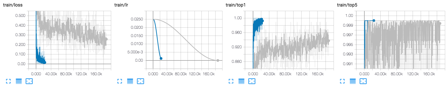
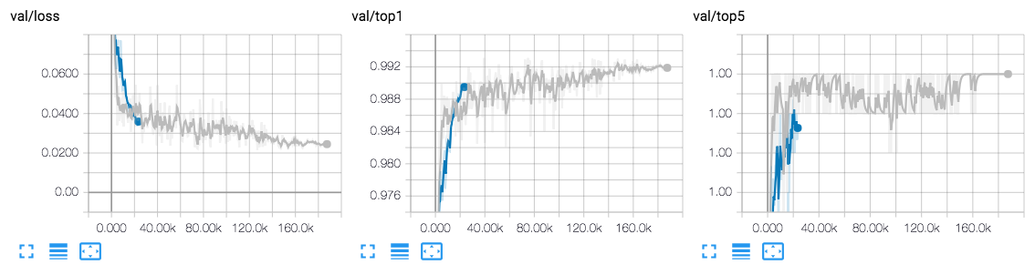
Fashion-MNIST 에 대한 TensorBoard 그래프다. 파란색이 search, 회색이 augment 에 해당한다. Search 는 50 epoch 을 돌고, augment 는 300 epoch 을 돌기 때문에 search 가 짧게 나온다.
Not covered here
본 튜토리얼에서 다루지 않은 내용이 몇 가지 있다:
- RNN
- RNN 은 여기서 따로 다루지 않았으며, github repo 에도 RNN 은 구현하지 않았다. 디테일한 부분을 제외하고는 동일하다.
- Tensorboard
- TensorboardX 를 사용해서 tensorboard 에 로그를 남길 수 있다.
- Visualize
- graphviz 를 사용해서 매 에퐄마다 찾은 구조를 시각화 할 수 있다.
RNN 부분을 제외하면 위 내용을 포함해서 디테일한 부분들은 github repo 에서 확인할 수 있다. RNN 이 궁금하다면 원 저자의 repo 를 참조하자.